
tl;dr – we can do much much better with our estimates of QoC or more accurately aQoC (and other factors) via some math, namely matrix algebra. Same with QoT or aQoT
So the topic of Quality of Competition (QoC) came up at the MIT Sloan Sports Analytics Conference recently and it has come up on twitter a couple of times since as well. Along with Quality of Teammates, there have been discussions along these lines since I joined the hockey analytics community via the yahoo group HAG (hockey analytics group) quite a while ago. And the issue, in my opinion, is framed the wrong way from a statistical viewpoint. Below I’ll discuss my, admittedly mathematical, approach to this.
The traditional way that hockey analytics refers to QoC and its partner Quality of Teammantes (QoT) is as single quantities. This suggests that what is being referred to can i get Aurogra without a prescription? is a single quantity. Generally across multiple games, it’s not a single quantity but it gets talked about that way. This approach results in unironic statements like ‘quality of competition doesn’t matter’. When you apply that to, say, facing a Capitals line of Ovechkin, Oshie, Backstrom, Alzner, Carlson versus the 3rd line for the Avs, it seems ridiculous. Of course, it is possible to amend the statement to say that on average QoC (aQoC) doesn’t matter. That statement might be true but the way that QoC and QoT are currently calculated won’t let us distangle all that stuff to be able to make that statement.
The notion of the value of Quality of Competition (QoC) or more explicitly average aQoC is a crude one. I’m not fond of QoC because the way that we should be dealing with assessing players is by estimating their impact on all of the events we are interested in http://thewoodlandretreat.com/home/the-bluebell-tent/dsc_0044-3/ simultaneously. The use of QoC comes from trying to analyze data at the player level rather than at the event level. The scale matters for data analysis. One tenet of Statistics, the discipline, is that your unit of analysis should be the largest unit that is impacted by your factors. In the case of sports that often means plays or shifts or possessions. Consequently, doing analysis at a game or season level is not ideal since it doesn’t disentangle all of the important impacts.
Since players skate against multiple opponents over the course of games, there is a need to address the impact of opponents on a player and the outcomes that results. One way to do this is to average those impacts, which is what most QoC do. And they do that by taking raw counts and averaging. The primary issue is that if you have players who are impacted by aQoC or aQoT effects then there raw numbers will have that impact and it will permeate your estimates unless you adjust for them. For example, Connor Sheary, when healthy, has been playing quite a bit with Sydney Crosby. If we are interested in Sheary’s aQoT for xG, then a calculation of that aQoT by averaging the individual player xG’s for his teammates weighting for event together will include Crosby’s xG impact. Now Crosby’s xG impact will include Sheary’s xG impact as well. If they are both players that impact xG positively then the aQoT xG for both players will be higher than reality since we have not extracted their individual impacts. That is, we need to have a way that extracts Crosby’s impact on xG (or any other outcome you want) while adjusting for Sheary and Hornqvist and Dumoulin and anyone
Could WOWY’s save us? Maybe, but then we will create a string of comparisons (Crosby without Sheary but with Kunitz, Crosby with Kunitz but without Sheary, Crosby with Sheary but without Cullen, Kunitz with Crosby but not Cullen, etc.) that is very hard to disentangle and adjust. And the thing about WOWY’s is that they assume everything else is equal when you make the with/without comparisons. Fortunately there is a better way.
It is possible to address QoC and QoT systematically at an appropriate level for analysis. One way to do this is through a multiple regression that has a term or terms for each players on the ice for a given event or shift. This area of research is known as adjusted plus-minus in the statistical analysis of sports literature. It is not easy to construct and can take some compute processing but it is the right methodology for this type of analysis. Begun by Rosenbaum (2004) (http://www.82games.com/comm30.htm) for basketball, examples using this framework has been published for hockey by Macdonald (2011, 2012), Gramacy et al. (2013), Schuckers and Curro (2013), and Thomas et al (2013). There is no need for an aQoC ora QoT to help with these approaches since these models explicitly assess and adjust for the impact of each player on each event or on each shift.
Here’s how this works for a game. Let’s consider how you might use regression to adjust for other players on the ice by looking at the play by play for Game 1 of the Stanley Cup Finals. Here is a link to that file: Game 1 2016 Stanley Cup Finals Play by Play file. See the screenshot below and note that the events are numbered in the first column on the left.
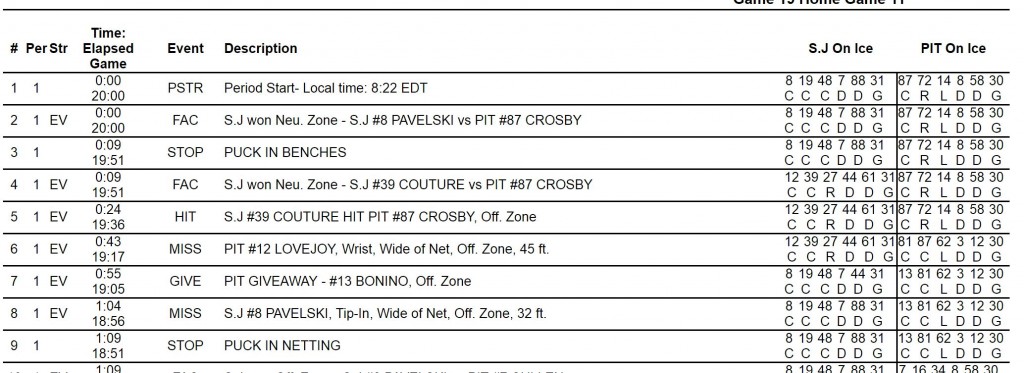
Table from NHL Play by Play events from Game 1 of the 2016 Stanley Cup Finals
The first action event (i.e. not a period start) is #2, a faceoff at neutral ice with SJ: Thornton, Pavelski, Hertl, Martin, Burns and Jones and PIT: Crosby, Hornqvist, Kunitz, Dumoulin, Letang and Murray. This is won by SJ and so value, if any for that event would be given to the SJ players and taken from the PIT players. Note that we record each player that is on the ice for that event.
Before the next faceoff (and after a stoppage which we will ignore), SJ makes a change and it is now Marleau, Couture, Donskoi, Vlasic, Braun and Jones, while PIT still has the list above. We would record the change of players in our data and credit/debit the appropriate players for being on the ice for the subsequent events, here a faceoff win by SJ and a hit by SJ.
The documenting of players on the ice usually takes the form of a row in a large matrix (called the design matrix, X) where each column is for a player who has appeared in a game and each row is an event or shift. If the player is on the ice they receive a 1 if playing for the home team and a -1 if playing for the away team. Thus, in the above sequence we would have 1’s for the SJ players and -1’s for the PIT players. For any player not on the ice, e.g. Malkin or Wingels, there would be a zero in their column for the rows of the events above. Malkin and Wingels will have non-zero values in their columns for later shifts in this game. If we were analyzing all of the playoffs in this manner we would have columns for players for DAL and TBL and they would have zero’s for this entire game. Thus at even strength we end up with 12 non-zero entries per row of our design matrix.
Back in Game 1, the Marleau line is out for three events (# 4 through 6) but PIT makes a change after the 2nd of these, though Crosby stays on the ice for the 3rd of these, #6. All of these plays are recorded as rows with players on the ice denoted by non-zero values in the appropriate columns. We continue the above for all of the relevant events in this game. Then we repeat the process for every game. For the analysis of an entire NHL regular season, there are about 1100 players and 250000 plays at even strength. Thus our design matrix will have 250000 rows and about 1100 columns. If we include special teams, there are another 50000 events. This is big data hockey analysis. By equating outcomes with impacts of players and other factors we have something like (n=) 250000 equations and (p=)1100 unknowns and we can solve that. Just a bit more complicated than your high school algebra of three equations and three unknowns, but a similar process for solving. Our solution, which are estimated player (and other factor) impacts, generally is one that finds a solution that minimizes the errors in those 250000 equations.
The assigning of values to the outcomes of on-ice events has been done a couple of ways. Macdonald (2011, 2012) — these analyses are now five plus years old — uses shifts and assigns values to shifts. That is, each row is a shift and the value of the row is the total value of that shift. Schuckers and Curro (2013) assigns value by play. Thomas, Ventura, Jensen and Ma (2013) looks at the rates of goal scoring by shift combinations and so as with Macdonald’s work the rows represent shifts or shift combinations of players. Gramacy et al (2013) use goals as success and saved shots. Not all of these methods use every event in the play-by-play files. For example, Macdonald does not use faceoffs in his models while Gramacy et al uses only shots.
All of the above methods start with work on even strength since that is the easiest to process but can be extended to account for special teams situations. In addition, we can have other terms in the model for score differential or for where a shift starts (zone starts) to account for those in our assessment of player impact.
Having defined the design matrix to have players from both teams, the resulting estimates of player impact via regression of the outcome metric with the columns of the design matrix accounted for their teammates and their opponents. The impacts of other players be they teammates or opponents are already in the estimates because they are already in the equations we are solving. The estimated player impact that we get is the average impact of that player on all the outcomes for which they were on the ice accounting for the players with them on the ice for all of those same events. That is, the methods deal with teammates and opponents on every event or every shift and, consequently, there is not a need to deal with aQoC or aQoT (or Zone Starts or Score Effects, etc) since they are built into the process. That said, it is possible to get values for average QoC and average QoT from the adjusted player estimates and the design matrix.
(Note none of the above regression adjusted plus minus methods for hockey use an ordinary least squares regression approach but they fundamental approach is similar.)
Optional Math Content
So it is possible to get an average QoC or QoT using the regression adjusted plus-minus framework that is part of the papers listed above. If we want to calculate QoC or QoT for these regression type models, we can. To do that define the design matrix as X, the outcome vector as Y and the estimated effects vector as q, where Y has length n and q has length p. Then we get estimated effects from
q = (X’X)-1X’Y. (1)
The X’X matrix is a p by p matrix (and I’m using ‘ (prime) to represent transpose of a matrix). Focusing on the terms for players only, each element contains the number of shifts or events when players are playing together. For event data, this is straightforward. (For responses that are rates there is a weighting that might need to be done but that can be done accommodated pretty easily with a weight matrix.)
To get aQoC let A be a truncated version of X’X where all of the positive elements of X’X are turned into zeroes. Then let a_k be the kth row of A. To get an average QoC for the player represented by the kth row of X’X, we would take the a_k*q/a_k*1_p where 1p is a vector of ones of length p.
To get aQoT let B be a truncated version of X’X where all of the negative elements of X’X are turned into zeroes. Then let b_j be the jth row of B. To get an average QoT for the player represented by the jth row of X’X, we would take the b_j*q/b_j*1_p where 1_p is a vector of ones of length p.
For the above, I’ve assumed that there are no other factors in X other than players. To get aQoC if there are other factors, the elements of a_k should be zeroed out for those entries. While I’m at it, we should be doing some sort of shrinkage rather than the ordinary least squares (OLS) in Equation (1). All of the aforementioned papers do this to improve their estimates of the impacts of these various factors, q.


Leave A Comment